Latency and Cost Are the Same Dial

Serving · June 13, 2026 · 9 min read

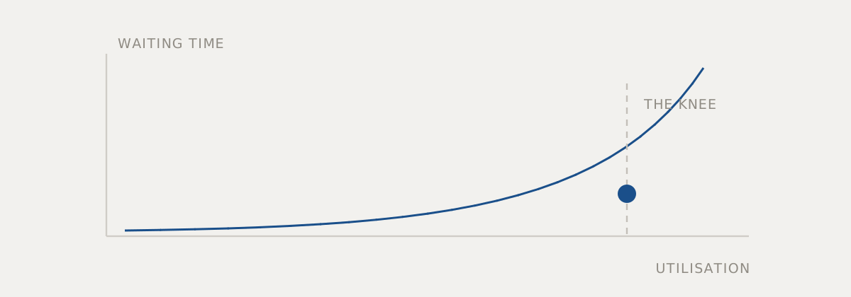
Two requirements arrive from different directions. Product wants responses faster. Finance wants the inference bill smaller. Both sound like independent engineering tasks, and a team can spend a quarter treating them that way before noticing that every improvement to one shows up as a regression in the other.

They are not independent. On a fixed fleet of accelerators, latency and cost per request are two readings from the same dial, and the dial is utilisation.

Where the money actually goes

Inference cost is dominated by the time an expensive device spends reserved for your workload, not by the number of requests that pass through it. A device sitting idle costs what a device running flat out costs. Cost per request is therefore total capacity divided by the work you managed to push through it.

That single fact explains most of the tension. To make each request cheap, you want the hardware busy — many requests resident at once, no idle gaps, high occupancy. To make each request fast, you want the hardware available the instant your request arrives, which is to say partly idle.

Anyone who has looked at a queueing curve knows what happens next. As utilisation climbs toward saturation, waiting time does not rise gently and proportionally. It rises slowly, then sharply, then vertically. The last increment of efficiency is bought with a disproportionate amount of delay, and the increment after that is bought with an outage.

Two different clocks

Discussing “latency” as one quantity hides the structure of the problem. A served request spends its time in distinct places, and they respond to different interventions.

Queue time is spent waiting for capacity. It is a function of arrival rate and available slots, and it is the component that explodes near saturation. You reduce it by adding capacity, shedding load, or admitting fewer concurrent requests — never by making the model faster.

Compute time is the work itself. For a generative workload it splits again: the initial pass over the input, which is compute-heavy and scales with input size, and the token-by-token generation that follows, which is limited by memory bandwidth and scales with output length. These two phases behave so differently under batching that treating them as one number will mislead every capacity calculation you do.

Overhead is everything else: network hops, serialisation, authentication, the gateway, the retrieval call, the safety check. It is often the largest single component in a system whose model is small, and it is invisible on any dashboard that only times the model call.

Optimising the wrong component is the most common wasted quarter in serving work. Before tuning a kernel, find out how much of the response time is queueing and how much never touched the accelerator at all.

Averages lie about queues

A median latency figure describes a system that is not under stress. It is measured mostly from requests that arrived when a slot was free, and it will look stable long after the tail has fallen apart.

The tail is where queueing lives, and the tail is what users experience as “it sometimes hangs”. Worse, the tail is where retries are born: a client times out, retries, and adds load to a system that was already saturated. A retry storm turns a slow period into an unavailable one, and it is entirely self-inflicted — the mechanism is a timeout set shorter than the tail the system can produce under load.

Set targets on the tail. Set client timeouts above it. Make retries back off, and cap them.

Streaming changes what “fast” means

For generated output, the response is not a single event. Perceived speed is governed by how quickly the first token appears and how steadily the rest follow; total completion time matters far less to a reader than either.

This is a genuinely free trade in some workloads. A configuration that starts producing output quickly and then generates at a comfortable reading pace can be substantially cheaper than one optimised for total completion, and users will report it as faster. It is not free for machine consumers — a downstream service parsing the whole output cares only about the final byte. One of the more useful things a serving layer can do is distinguish the two classes of caller and stop holding them to a single target.

Capacity is bought in whole units

Accelerators are not fluid. You reserve them in discrete pieces, and a model’s weights must be resident before any request can be served, which means a replica that exists at all costs full price whether it handles one request per minute or thousands.

Two consequences follow. First, low-volume models are expensive per request for reasons that have nothing to do with efficiency, and the answer is usually consolidation rather than tuning. Second, autoscaling responds slower than traffic does, because a new replica must be scheduled, the weights must be loaded, and any warm-up must complete. If that takes minutes and your traffic spikes in seconds, scaling is a cost-control mechanism, not a latency-protection mechanism. Latency protection under a spike comes from headroom you were already paying for, or from shedding load deliberately.

Deciding rather than drifting

The useful framing for capacity is an explicit choice, written down: this workload runs at high occupancy and accepts queueing, that one runs with headroom and accepts the cost. Batch scoring, background enrichment and internal tooling belong in the first category. Anything a person is waiting on belongs in the second.

Mixing both classes on the same replicas without prioritisation gives you the worst of each — the interactive traffic inherits the queue depth of the bulk traffic, and the bulk traffic gets throttled for the sake of latency it does not need. Separation, either by fleet or by an admission policy that understands priority, recovers most of the loss.

The arithmetic here is not complicated, and it is worth doing before the architecture rather than after. Requests per second, tokens per request, throughput per replica, and the latency you have promised — those four numbers determine your fleet size and your bill, and they will not stop determining them because a proposal assumed otherwise. The inference cost estimator on this site runs exactly that arithmetic with your own figures, so the trade is visible before it becomes an invoice.