Drift Is a Question, Not an Alarm

Monitoring · July 10, 2026 · 9 min read

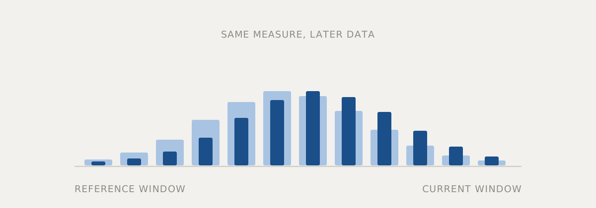
The dashboard turns amber. A distribution test on one of the input features has crossed its threshold. Somebody opens the runbook, which says: investigate drift.

Three hours later the finding is that a client application changed its default sort order, so a categorical feature shifted its proportions. The model’s accuracy is unchanged. The alert was correct, in the narrow sense that the distribution really did move, and useless in every sense that matters.

Repeat this a dozen times and the amber tile stops being read. The monitoring did not fail because the statistics were wrong. It failed because a statistic about inputs was treated as a statement about quality.

What each kind of drift can and cannot tell you

It is worth separating the phenomena, because they have different diagnostic value.

Input drift means the distribution of features has changed. It is easy to measure, requires no labels, and is available immediately. It also correlates weakly with harm: models are frequently robust to substantial input movement, and occasionally very fragile to a small one. On its own it tells you that something upstream changed — nothing more.

Prediction drift means the distribution of the model’s outputs has changed. Also cheap, also label-free, and rather more informative, because it reflects how the model responded to whatever moved. A sharp change in the rate of a particular predicted class is worth looking at within the hour.

Concept drift means the relationship between inputs and the correct answer has changed — the same input now warrants a different output. This is the only one that reliably degrades a model, and it is the one you cannot see without labels.

The awkward consequence is that the cheap signals are the weak ones and the strong signal arrives late, sometimes very late. Any monitoring design is essentially a strategy for handling that asymmetry.

Data quality masquerades as drift

Before treating any distribution shift as a modelling phenomenon, rule out the boring explanations, because most alerts are boring.

An upstream job failed and a feature is now null for a slice of traffic — often imputed silently to a default that the model reads as a real value. A schema change altered units, or a currency, or a timezone. An enrichment service started timing out and returning fallbacks. A new client integrated and does not populate an optional field the model leans on heavily.

None of these are drift. They are bugs, and they are far more common than genuine concept change. Checks for nullity, cardinality, range and freshness on each feature will catch them faster and more specifically than any distributional distance, and they produce alerts an engineer can act on without a modelling discussion.

Build those first. A team that adds distribution monitoring before input validation will spend its first year investigating outages in the disguise of statistics.

The label delay problem

The honest measurement of a model’s quality requires knowing what actually happened. Sometimes that takes seconds; often it takes weeks; sometimes it never arrives for the cases you care most about.

Worse, the labels that do arrive are usually not a random sample. If the model’s prediction determines the action, then outcomes are observed only for the actions taken. A fraud model that blocks a transaction never learns whether it would have been fraudulent. A recommender only observes engagement with what it chose to show. Feeding those observations straight back into training teaches the model that its own past decisions were correct — a loop that tightens quietly and looks like improving metrics the whole way down.

Some of this is recoverable. A small, deliberately randomised holdout of traffic that bypasses the model produces unbiased outcome data at a known cost. Where randomisation is not acceptable, logging the model’s confidence alongside the decision at least allows reweighting later. What does not work is pretending the observed outcomes are representative.

What should actually trigger a retrain

Given all that, the trigger worth wiring up is degradation in an outcome you believe, measured on a population you did not select. Everything else is a prompt to investigate.

That leaves a gap while labels are pending, and the gap is best filled by a schedule rather than a statistic. Regular retraining on fresh data has properties that trigger-based retraining lacks: it is predictable, its cost is budgeted, the pipeline is exercised often enough to still work when needed, and it does not create an incentive to tune thresholds until the alarms stop.

Choosing the cadence is a matter of how fast the world moves for your problem. The test is empirical and cheap: train a model as of a date in the past, evaluate it on each subsequent week, and watch how the curve decays. If it holds flat for months, weekly retraining is expensive theatre. If it decays within days, no monitoring strategy will save a monthly cadence.

Retraining is a deployment, not a refresh

The most damaging habit in this area is treating an automatically retrained model as safe because it used the same code. It is a new model. It can be worse. It can be worse in one segment while improving overall, and if it is deployed without evaluation, that regression ships unobserved.

Every retrained candidate goes through the same gate as a hand-built one: evaluation on the stable set, slice-level comparison against the incumbent, shadow traffic if the stakes justify it, then a staged rollout with the ability to revert. Automation should shorten that path, not remove it.

And when the pipeline retrains on data the current model influenced, record that fact in the lineage. The generation number of a model trained on its predecessor’s decisions is a useful thing to know before anyone tries to explain why the system has become confidently strange.